Strengthening learning is becoming more scalable, with efficiency becoming a key variable
When pre-training brings the big model to the starting point of new capabilities, reinforcement learning determines how far the models can go by continuous exploration and feedback, continuously stimulating their reasoning and action skills in new environments and new tasks.
The greater the role of RL in model development, the more direct the impact of training efficiency on the computational budget.
For example, suppose 10 GPUs run continuously for 30 days, at $3 per hour per card, the total cost is $21.6 million. If you use the same number of cards, achieve the same model effect, but reduce the training time by 10%, you can use 720,000 GPU hours less, saving about $2.6 million.
One of the most basic parameters that almost all training formulations cannot bypass is Batch Size.
In practical training, Batch Size often occurs in two types of decisions:
Batch Size Tuning: Allows the formulation to adapt to new conditions. Models are enlarged, or GPU card types are changed, and the original Batch and learning rate are not necessarily the same. Batch size is too small to make the hardware inadequate, and unmatched learning rates can cause learning to slow down or even become unstable.
Batch Size Scaling: Turning parallels into shorter training times. If the same model gets more GPUs, can the Batch synchronize to allow the model to scale earlier? Even if the number of GPUs does not change, if the synchronous generation is lower, is the device not working properly, can the larger Batch take advantage of this part of the dormant capability?
Both types of decisions ultimately lead to the same real question: How to find the best Batch Size to get the model to perform in the shortest time possible?
A larger Batch, which could be both an accelerator and a slow-speed belt. The Tencent mixing team observed in the experiment: Moderately increasing the Batch, and simultaneously adjusting the learning rate, can improve the throughput while maintaining learning efficiency; but when the Batch is too large, the additional sample cost will in turn overwhelm the throughput yield.
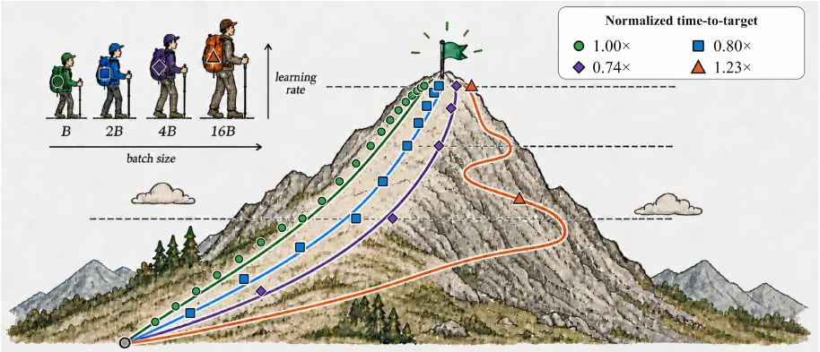
Figure 1 compares training to mountaineering: the peak represents the same target performance, the four routes represent different Batch Sizes, and each path indicator represents an optimised update. Following the supporting adjustment learning rate, B, 2B and 4B maintain the same learning progress in the cumulative sample dimension; the larger Batch "climbs" because of higher and faster throughput. But after expanding to 16B, the sample efficiency losses exceed throughput yields, climbing instead slower than B.
What is the scientific law behind this shift from acceleration to deceleration? Can a set of measurable guidelines be established to find the shortest time-to-target Batch Size?
To answer this question, the Tencent Mixed Team re-examined the scale laws of big model reinforcement learning, starting from the principle of primacy in the common constraint of Batch Size training dynamics and hardware execution.
When Do Larger Batches Help Scale LLM Reinforcement Learning?
Tencent Hy Team (also known as Tencent Hy Team)
The following is a link to article: arXiv:2608.29296
From Classic Batch Scaling to LLM Reinforcement
"To what extent can batch be expanded effectively?" is not a new question.
In 2017, the value of Big Batch first came to the public's attention in an engineering breakthrough. Priya Goyal, Yangqing Jia and Kaiming He of Facebook, among others, in their Accurate, Large Minibatch SGD: Training ImageNet in 1 Hour series, through linear drop-out rates and gradual warmup, increased ResNet-50 training on ImageNet from 8 GPUs, Batch 256 for about 29 hours, to 256 GPUs, Batch 8192 for 1 hour, while maintaining the accuracy of the small Batch.
This work demonstrates that, with supporting optimization, a larger Batch can indeed convert more hardware in parallel to shorter wall-clock time; it also pushes the question from "can Big Batch train" to "how effectively can Big Batch scale".
In 2018, Sam McCandlish, Jared Kaplan, and Dario Amodei, current CEO of Anthropic, at OpenAI, investigated when the benefits of extended batch training began to decrease, and linked this turnover to gradient noise measurement. Later, Christopher J. Shallue and George E. Dahl of Google Brain further pointed out that the effective benefits of data parallelism depend on specific tasks, and fairly on the need to adjust the hyperparameters for different batches respectively.
Another closely related question is Batch Size Invariance: Will the model maintain an approximate learning trajectory while consuming the same number of samples if superparameters such as adjustment learning rate are supported after changing Batch? In 2022, Jacob Hilton, Karl Cobbe, and John Schulman of OpenAI conducted a systematic study of this problem in strategy optimization.
So what's so special about LLM reinforcement learning?
In supervised learning, training samples are usually stored in fixed data centers. After extracting a larger Batch, the main additional costs occur in the forward propagation, reverse propagation and parameter updates of the model; the sample itself does not need to be produced by the model being trained. Therefore, classic Batch Scaling mainly discusses how the larger Batch can change gradient estimates, update frequency and training parallels.
LLM reinforcement learning has another key closing loop. As an Agent, Transformers must first use current strategies for self-generation, or continuous interaction with the environment, to get answers, trajectories, and rewards; these online-generated data then enter the learning phase for forward propagation, reverse propagation, and parameter updates.
In other words, models are both a reasoning system for producing training data and a learning system for consuming that data.

The two main computational components of LLM reinforcement learning rely on GPUs: sampling to generate responses and trajectories through automated regression reasoning, and training using these data update models. The "pathway" connecting the two sides to the GPU is shaped by Batch Size: it affects both the sampling side's concurrent scale and the amount of data processed by the training side each update.
From a system architecture point of view, although the two processes run on the same Transformer, they are different from the way GPUs are used. Generating is a token-by-token self-return logic that requires repeatedly reading the model weight, maintaining the KV Cache and scheduling and sequencing; learning performs forward and reverse propagation on the entire batch of tokens, while also preserving activation, computing gradients and updating optimizer status.
Therefore, Batch expansion is not just about adding more data to the same computation: it can both increase production efficiency and increase computation and storage costs on the training side by simultaneously increasing production efficiency. The learning curve cannot independently answer how fast the training will be, and the generation throughput cannot independently answer how many samples the model will need.
Two efficiencies, one analytical framework
For large-scale model training, the ultimate goal is not to get the Batch to the maximum or to get a local stage to run as fast as possible, but to get the model to the required capability level as soon as possible. The paper uses Time-to-Target to measure this goal: from the start of the training to the first time the model reaches the default verification goal, how much time has actually passed.
The speed of the scale is determined jointly by two efficiencies:
Sample efficiency: How much learning progress each training response brings. Batch Size and its accompanying hyperparameters change learning outcomes under a fixed sample budget.
System efficiency: how many training responses are generated and processed per second by the entire training stream, including the cost of generating, updating models, and waiting and synchronizing.
If J represents verification performance, N represents cumulative training responses, and t represents real time. Along a smooth, approximate learning path, there are:
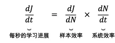
If the throughput is doubled, but the learning progress of each response falls by half, both are offset. In order to make an operable comparison in experiments with greater noise and only in discrete checkpoint assessments, the paper further fixes a verification goal. The average end-to-end throughput of q over this period is:
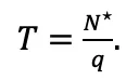
For reference configurations, the ratio of the number of samples reached is marked as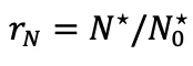 The ratio of end-to-end ingestion is recorded as
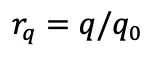 Among them,
 This is the "sample cost" that indicates the need for more responses.
 The answer to this question is to "swallow profits" and to "process more responses per second".
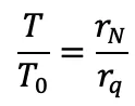
This relationship offers two perspectives:
In theory, the net proceeds are compared to the sample cost.
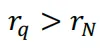 This means that the larger batch will make the training faster when the increase in throughput exceeds the increase in the number of samples.
In practice, first establishing consistency and then optimizing throughput. First rearranging the batch-related hyperparameters to find a batch area "nearly aligned with the learning curve drawn by the cumulative sample number".
 As long as
 Improving end-to-end throughput can reduce the time it takes to reach the target more directly. If system optimization changes learning behavior, it is necessary to re-check whether this alignment is still in place.
Takeaway:
Batch Size simultaneously affects the learning progress of each response, as well as the end-to-end throughput of the system processing these responses.
The larger Batch will shorten training time only when the throughput yield exceeds the incremental sample size.
A simpler practical path is to build an approximate Batch Size Invariance and then optimize the throughput within this range.
Step 1: Keep the learning effect of each sample
Batch Size Invariance has a very direct meaning: if the batch is doubled, the number of optimizer updates required for the model to achieve the same effect should be reduced by about half, so the total sample demand remains essentially unchanged.
In other words, a fair comparison that is reasonable and consistent with the Scaling intuition should be satisfied after the supporting hyperparameters for different Batch individually adjusted learning rates: more samples will produce better performance, while the cumulative consumption of the same number of samples will result in approximately the same performance for different Batches.
But this doesn't happen automatically: larger batches use more response averages, but also lose some updating opportunities within the model's fixed sample budget. To maintain the learning effect of each sample, it is necessary to rearrange how far each update goes.
For Adam Optimizer, the team used the square root rule as the starting point for adjusting the learning rate:
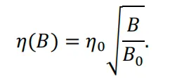
This rule is only a starting point and needs to be experimentally verified. The paper only changes the learning rate, keeping other optimizer hyperparameters unchanged; joint adjustment of more hyperparameters may further improve the immutability, but this remains for further research.
To make this comparison as straightforward as possible, the paper evaluated GRPO and PPO in a self-development training system. Both types of experiments performed only one global optimizer update per rollout batch, did not dismantle the minibatch, and did not reuse the rollout, thus avoiding the introduction of additional modulation dimensions such as minibatch size and optimized epoch.
Finding one: GRPO is almost constant within 16 times the prompt batch.
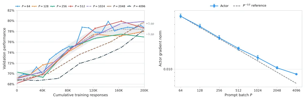
Figure 3 shows that after adjusting the learning rate below the fixed group size, the GRPO shows an approximate aligned learning curve within a boundary range. The largest groups of Batch begin to deviate and the decline in the actor gradient range also slows down. The gray ±1 percentage point range is only a visual reference, not a confidence interval. Source: paper Figure 2.
The paper conducted a GRPO training on Qwen 3-30B-A3B-Instruct-2507, with data from the filtered DAPO-MATH-17K, and an average mean@32 evaluation of AIME 2024 and AIME 2025. Here, a training sample refers to responses that have been filtered, actually retained and used for optimizer updates; an update contains P prompt group, each group with a G line, so that =PG. When G=8, the adjusted learning rate runs from P=64 to P=1024, showing a similar sample learning curve in the window; and when P=2048 and P=4096, the curve falls below this family.
The graph to the right provides a complementary view of this deviation. Decline; at P=2048 and P=4096, this decline begins to slow, and no longer appears simultaneously with the learning curve in the left graph. This is consistent with the marginal gain decline of gradient averages; but gradient parameters are only indirectly diagnosed and cannot alone prove the cause of the invariant disruption.
Discover 2: The scale of the actor and the critic in the PPO is different
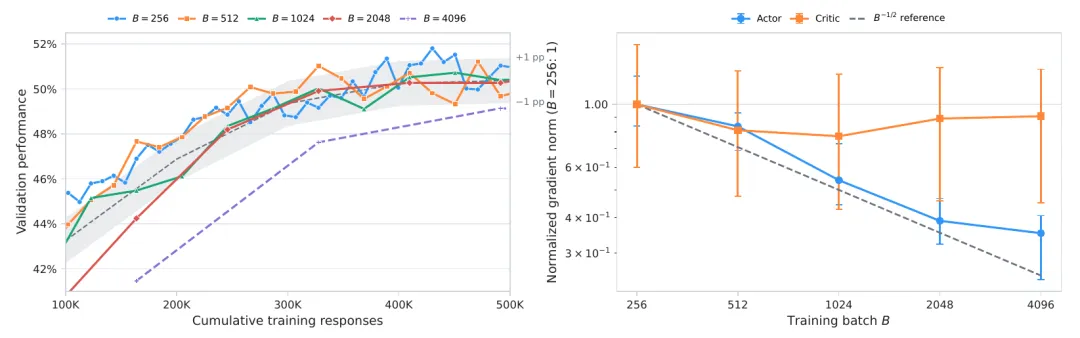
Batch Scaling in Figure 4 of the PPO. The left-hand graph shows the relationship between the verification performance and the cumulative number of trained responses; the right-hand graph shows the change in the actor and critic gradient parameters with the Batch. The sample axis excludes the initial 30 steps of warm-up of the only trained critic, and starts counting the training time from the actor.
The PPO experiment uses an internal mixing strategy model and a value model, both of which are 3B activation parameters, with training data mixing mathematical, scientific, and logical tasks, and evaluating scores as the average performance of the corresponding benchmarks. In this setting, each prompt retains only one answer, namely G=1,=P.
The graph on the right shows the difference between actor and critic. As the batch increases, the actor gradient spectrum continues to decline, which tends to ease in the largest batch; the critical gradient spectrum is relatively flat and fluctuates more. Because the two have different training objectives, they may have different effective batch scales, which can be considered in the future for analysis and optimization respectively.
Figure 3: Batch of GRPO should look at total responses
In GRPO, Batch expansion has two directions: to increase the number of prompt, or to increase the number of responses to each prompt. Larger responses Batch can reduce gradient estimate differences by averaging more samples, but these two paths are not exactly equivalent: responses within the same group share the prompt, and build advantage through relative rewards within the group.
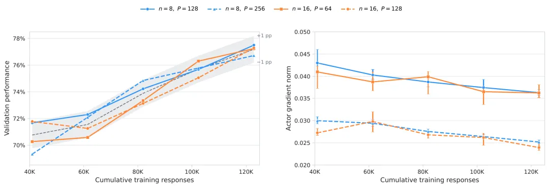
Figure 5 shows the group-size comparison of the GRPO. The left is the relationship between the verification performance and the cumulative number of training responses; the right is the actor gradient parameter in the same training window. The real line corresponds to 1024 responses per update, and the empty line corresponds to 2048; the blue and orange represent group sizes of 8 and 16 respectively.
The paper compares two sets of total Batch configurations: ((P,G) = ((128,8) and (64,16) with 1024 replies each update; ((256,8) and (128,16) with 2048 replies.
In the diagram on the left, the same configurations of the total answer numbers show roughly similar learning trajectories, although they are not completely overlapping at each checkpoint. The pairings on the right are clearer: the total answer Batch at the same time, the actor gradient parameter is also close; while the gradient norm in the 2048 answer is always smaller than the 1024 line. These results support the use of =PG as a Batch unit of GRPO in the already measured configuration, but cannot therefore be assumed that the prompt number and the group size are interchangeable under any set.
Discovering Four: Keeping learning unchanged destroys approximate consistency
In practice, adding GPUs tends to simultaneously extend the parallelity of the data and the overall Batch. If parameters such as learning rate are still configured along the smaller Batch, training may not necessarily be distributed, or even appear more smooth because of the smaller gradient noise. However, when the same number of responses are consumed, the smaller number of parameters updated by the larger Batch does not necessarily achieve parity.
In other words, training stability does not mean that Batch Size Invariance is still in place; it may require more responses to keep up with the smaller Batch.
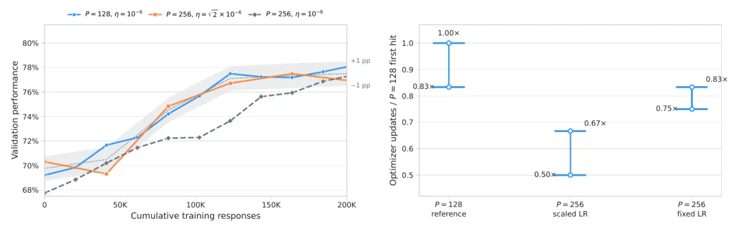
Figure 6 shows a comparison of the learning rate of the GRPO. The left shows a reference Batch, a quadrupled Batch after adjusting the square root learning rate, and a quadrupled Batch that keeps the learning rate unchanged. The right shows the number of updates required to achieve the goal and is unified by reference configuration. The endpoint range reflects the granularity of the evaluated checkpoint, not the confidence range.
The team used P=128 as a reference, and compared two P=256 configurations: one adjusted the learning rate and the other remained the same with the group size. In the left, the large batch after adjusting the learning rate generally follows the reference curve; the operation of the fixed learning rate was significantly lagging behind during most of the training. For example, the latter accounted for about 74% of the cumulative 120,000 responses, while the reference and adjusted operation accounted for about 77%.
The graph on the right further quantifies the number of updates. If the Batch Size Invariance is accurate, the number of updates after the Batch doubled should be 0.50 times the reference configuration. The adjusted learning rate configuration is 0.50 times 0.67 times, which is basically consistent with this ideal value; the fixed learning rate configuration requires updates of 0.75 times 0.83 times.
Takeaway:
After re-adjusting the learning rate, both GRPO and PPO only showed approximate Batch Size Invariance within a certain Batch; the Batch continued to grow and the sample-level learning curve began to deviate.
GRPO's group-size comparison illustrates that in configurations that have been measured, the overall Batch response is more capable of depicting learning behaviour than the prompt number or group size alone.
In PPO, actor and critic are not on the same scale.
Contrasting fixed learning rates further demonstrates that training stability is not the same as consistency.
Step 2: Increase throughput on fixed hardware
The next question is how to process the samples more quickly after each sample has been approximated. A common practice is to increase the GPU and expand the data in parallel; but if the amount of hardware does not change, can the larger batch also be accelerated?
Production phase: From regression decoding, a new token is generated for only one sequence each time. When the concurrency is lower, GPUs need to repeatedly read the model weight, but only process a small number of token vectors.
Training phase: Once a response has been generated, forward and reverse propagation can handle a large number of token locations simultaneously, exposing a higher parallelism. In this case, increasing the Batch is mainly an increase in workload. In the GRPO configuration of the paper measurement, the prompt batch doubles from 128 to 256 and the actor update time increases from 101.3 seconds to 208.6 seconds, basically an increase in the proportion to the Batch.
A simplified local model can describe this difference:
In this case, the number of responses in the logical rollout batch represents the number of reserved responses that an optimizer uses to update its consumption. The paper experiment uses asynchronous partial rollout, and so the expansion of the training batch will also simultaneously expand the production of the batch.
The paper further explains this intuition from a Roofline perspective: Batching changes the strength of the algorithm, or changes the execution in the memory bandwidth bottleneck or computational bottleneck. The simplified model above summarizes the cost difference between generating and training.
Figure 5: On fixed hardware, generating time increases in linear ways.
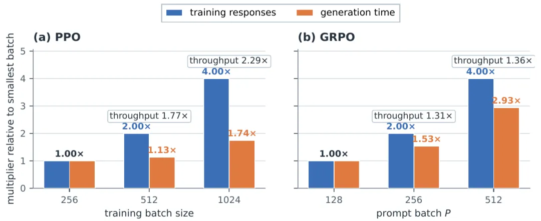
Figure 7 On fixed hardware, more responses do not necessarily need to increase the collection time proportionally. When the batch increases fourfold, the generation phase throughput of the PPO increases to 2.29 times and the GRPO increases to 1.36 times. These are measurements of the generation phase, not end-to-end training acceleration. Source: paper Figure 6.
Figure 7 simultaneously shows the multiples of the response number and the collection time relative to the smallest Batch; the blue response number increases faster than the orange response time, and the ratio of the two is the generation phase throughput yield. In PPO, the training Batch increased from 256 to 1024, the response number increased fourfold, while the collection time increased from only 39 seconds to 68 seconds, so the response collection throughput increased to 4/68/39) = 2.29×.
In the GRPO, P increased production phase throughput by 1.31 times from 128 to 256; increased to 512 increased by 1.36 times. Additional gains from 256 to 512 have been small, indicating that, within the measured range, utilisable generation throughput gains are trending toward saturation.
The conclusion of the phase:
There is a computational asymmetry between generation and training in LLM reinforcement learning: generation is easier to read with weight and memory bandwidth constraints, while training has been exposed to higher parallelism and time-consuming closer to linear Batch growth.
Larger batches can allow more sequences being decoded to allocate weight-to-reading costs, thus increasing generation throughput even on fixed hardware.
Step 3: Combine two Critical Batches to find the shortest Time-to-Target
The above results reveal the two distinct boundaries of Batch Scaling in LLM reinforcement learning:
Critical generation batch is about system efficiency: for fixed models, decoding engines, answering length distributions and hardware allocations, it marks the location of the generation of throughput near the platform. Prior to this, larger batches would improve hardware utilization; after that, continued expansion would yield little generation throughput gain.
Critical training batch is about sample efficiency: it is close to the upper limit of Batch Size Invariance under the current recruitment program. Prior to that, larger Batches needed roughly the same number of responses to reach the same goal; beyond this range, the average return of more responses was no longer enough to fully compensate for fewer updates, and the demand for batch sizes began to increase.
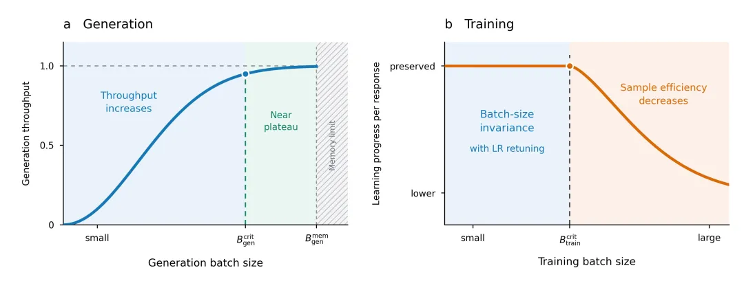
Figure 8: There are two critical batches. Figure 8: Generating throughput as the Batch increases gradually closer to the platform, with the display capacity constituting an independent feasibility constraint. Figure 8: After adjusting the learning rate, the learning effect of each response remains approximate within a range and then decreases in the larger Batch.
The two boundaries are separated because they answer two different questions: how much hardware can be mined by the generation side, and whether the training side can retain the learning effect of each response. The storage capacity may also limit the available Batch before it reaches the throughput platform. But neither boundary can give the fastest configuration separately: if the generation Batch and the training Batch increase along the same scale B, their relative sequence will form a different timestamp curve through a balance between "sample cost, end-to-end throughput".
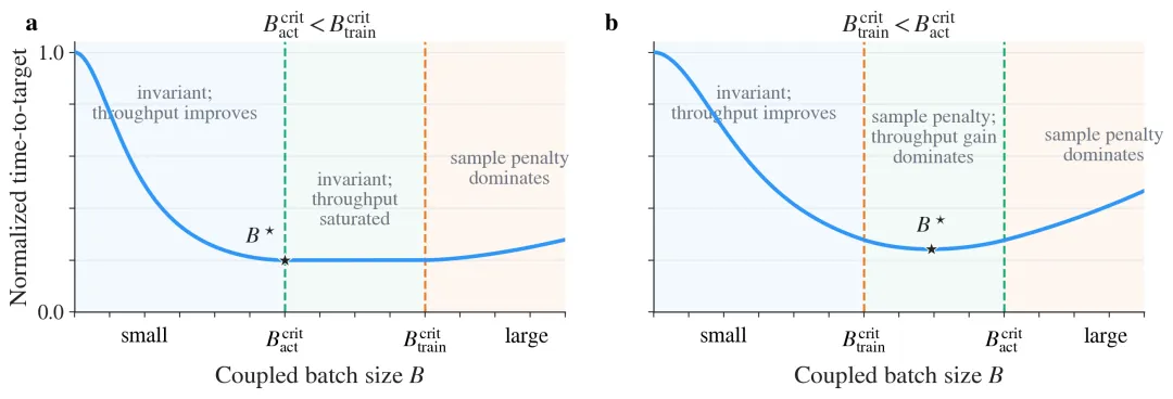
Figure 9: When Batch generation and Batch training are connected, there are two possible scenarios for time-to-target expansion. Figure 9: The generation of throughput precursors and the emergence of an approximate optimum platform before the start of the sample efficiency decline. Figure 9: The learning efficiency decreases, but the throughput gains temporarily compensate for the additional sample, thus indicating that it is best to stay out of the same range.
Figure 9 can be divided into three operating zones:
The learning effect is maintained and the throughput is still improved: the number of responses required by model scales remains largely unchanged, but the system can process them faster, thus reducing training time.
The learning effect is maintained, the absorption is saturated and: continuing to expand the Batch has been difficult to bring in additional speed gains, so a batch interval may have similar training time.
The cost of extra samples is skyrocketing: once a larger batch requires more responses to reach the target, limited throughput increases cannot be compensated, and training time increases again.
Of course, the order of the two boundaries can be reversed. If learning efficiency deteriorates first, but production throughput also improves rapidly, then as long as throughput gains are greater than the additional sample cost, larger batches may still be faster. Therefore, the ultimate goal is to minimize time-to-target, rather than mechanically selecting a critical batch.
Test results: The best configuration is shortened by 29%, the worst is slower by 42%
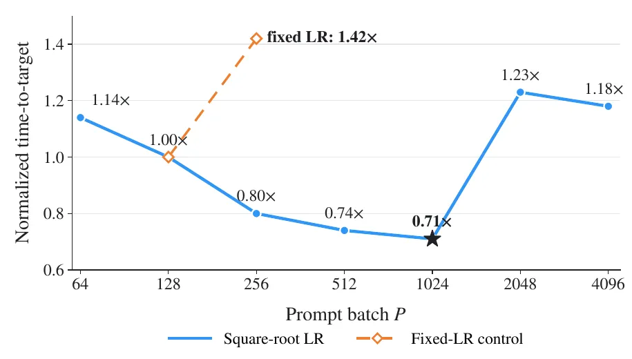
Each prompt generates 8 responses, with blue points using square root learning rate Scaling, orange controls keeping the learning rate unchanged; all times are referenced with P=128 for unification, with a star sign indicating the best of the configuration. Source: paper Figure 8.
After re-adjusting the learning rate, P was increased from 128 to 512 and 1024, and time-to-target was reduced to 0.74 times and 0.71 times, respectively. At P=1024, the model and reference configuration, with 122.88K, kept the answer to the target, increased end-to-end throughput by 41%, and training time decreased from 11.90 hours to 8.42 hours, i.e. without increasing the GPU, and the target time was reduced by 29%.
But the larger Batch is not always better. At P=2048 and P=4096, the number of responses required by the DAC increased by about 60%, exceeding 30% and 36% of the throughput yield, and the final training time increased by 1.23 times and 1.18 times. Even in medium-sized Batches like P=256, if the learning rate remains unchanged, the throughput only increases by 17%, the DAC response rate increases by 67%, and the training time becomes 1.42 times the reference configuration.
To put the previous judgments into practice, it can be compressed into two steps:
Coordinated learning outcomes: Adjusting the learning rate for each candidate's batch training, comparing the learning curve under the same cumulative answer numbers, and estimating the cost of a benchmark sample.
Comparison of system benefits: Adjusting Batch generation or decoding concurrently to the extent permitted by high storage, measuring end-to-end throughput q, and finally selectively configuring and confirming that it can reach its target sooner.
The Batch Optimization Framework in Algorithm 1's paper: First adjust the learning rate and estimate the cost of the benchmark sample, then look for the end-to-end throughput gains generated by the synchronization, and finally select the configuration according to the benchmark time.
Significance and boundaries of this work
The value of this work is not in proposing a new reinforcement learning algorithm, but in providing a simple, scalable and hardware-aware way of thinking for existing GRPO and PPO training.
Theoretical understanding: Why does batch get bigger and why can't it keep getting bigger?
The study broke down two previously easy-to-mix problems: models can't learn as well using the same number of trained samples; these samples can't be processed faster on a given hardware. Learning Rate Scaling can maintain an approximate Batch Size Invariance to a certain extent, but this rule will ultimately fail.
Training Practice: First confirm that you've learned well, then figure out how to run fast.
When changing the training Batch of GRPO or PPO, the adjustment learning rate should first be accompanied by checking if the same cumulative response number can achieve a similar effect; then improving the synchronization generation, measuring real end-to-end throughput. After changing the model, changing the task or changing the hardware, this adjustment sequence can be repeated, but cannot directly move the Batch values obtained once.
System design: Determine the cost of production and training, and decide how to expand the Batch.
Production phases are usually subject to weight-reading and memory bandwidth constraints, with higher concurrent allocation of this part of the cost; the higher the arithmetic intensity of the training phase, the larger Batch optimizer does not necessarily bring the same benefits. Therefore, Batch generation and Batch training do not necessarily have to be simultaneously expanded.
How to evaluate: different batches must be compared on the same runway.
The groups first adjusted the batch-dependent configuration, and then looked at two issues: using the same number of samples, who learned better; reaching the same ability goal, who spent less time. Comparing the same scores after updating the number of steps could make "seeing more samples" a "learner" mistake; and comparing "processing faster" could make "training completed sooner".
These conclusions also have clear boundaries. When models, rewards, task distributions, training phases, reasoning engines, or execution strategies change, both sample efficiency and system throughput may change, and the effective Batch range that has been measured cannot be directly illuminated. A natural next step is to move beyond the current setting of "learning-only modulation" to look for other Batch-dependent hyperparameters; the PPO experiment also suggests that actors and critics may need different Batch scales.