Core conclusion: The four residual flows of the mHC are not used in a uniform manner. The read-write weight is concentrated on about two flows; deep ((22×42 layers) residual mixing has approached the unit matrix. Intervention experiments show: removing the weakest read-write path, the six-mission average decreases by a maximum of 0.38 percentage points, and the six-mission average remains essentially unchanged after the deep residual mixing matrix is replaced by the unit matrix.

How does mHC use its residual streams? Selective Routing and Near-Identity Mixing
Link to the paper:https://arxiv.org/html/2609.05309v1
DeepSeek-V4-Flash uses the mHC structure to maintain four residual flows, but they are not used uniformly in actual computation. The mHC generates read-write weights for each token separately, so the routing can change with input. However, in the trained model, the same sublayer dominant flow selection shows stronger consistency with the token: for the same Attention or FFN sublayer, the read-write weights are usually concentrated on about two residual flows.
We further intervened in the reasoning phase, removing the smallest path of reading or writing weights for each token, respectively, where the PPL rose to a maximum of 2.7%, and the average score for six tasks decreased to a maximum of 0.38 percentage points. After replacing the residual mixed matrix of the 22nd and 42nd layers as a unit matrix, the PPL rose to 1.9%, and the task average remained essentially unchanged.
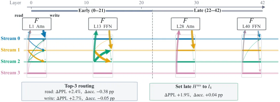
In Figure 1, the read-write of the quadratic mHC is mainly concentrated on a few residual flows, with the dominant flow switching with depth; the shallow layer retains the cross-flow mix, while the deep layer passes close to each flow independently.
From single-flow residues to multi-flow residues
In the standard Transformer, each Attention or FFN sublayer reads the hidden state from the same residual flow and adds the calculation results to this flow. Hyper-Connections (HC) and Manifold-Constrained Hyper-Connections (mHC) extend the single residual flow into multiple parallel streams.
In the DeepSeek-V4-Flash model analyzed in this article, the mHC maintains four residual flows. The input residual flow of an Attention or FFN sublayer is marked as
 The sub-layer is updated to:
For a single token,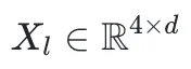 where d is the dimension of the hidden state. Read mapping and write mapping by line vector respectively
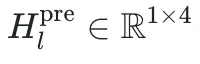 and
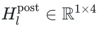 Indicates residual mixed mapping by matrix
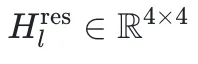 All three maps use input-dependent parameterization: the model generates a read-write-weight and residual mixed matrix using learning parameters based on the hidden state of the current token in the sublayer.
 For its parameters.
The mHC also uses the Sinkhorn Knopp inversion pair to unify it into a binary random matrix, i.e. the sum of the nonnegative elements per row and each column is equal to 1, to improve training stability. The unit matrix also meets this restriction, and when it approaches the unit matrix, the streams pass independently mainly along the residual path. However, the mHC is not directly fixed as a unit matrix, retaining the ability to mix dynamically.
The mHC allows the model to adjust the read-write and mix modes of the four residual flows with input, but it is not clear how the post-training model uses these flows and to what extent it relies on this dynamics. Therefore, we analyzed the impact of the DeepSeek-V4-Flash forward-computing read-write weights, residual mixed matrix and the hidden states of the streams on the model's performance by reasoning interventions, checking read-cutting paths, or replacing residual mixed matrix.
Analysis of objects and assessment settings
We used open DeepSeek-V4-Flash-0731 weights to analyze. We randomly sampled 512 sequences of 1,024 lengths from C4 data sets and recorded a mixed matrix of read-write weights and residuals generated by each token in a forward computation to observe changes in these maps with input and network depth. We also evaluated the performance of the intervening model using C4 data set confusion (PPL) and six zero-sample tasks (ARC-Easy,ARC-Challenge, PIQA, HellaSwag, MMLU, and GSM8K).
The concentration of read-write routing and the choice of dominant streams
Read the map. And write a map.
 Determine from which residual flows each sublayer reads and writes to which residual flows. For each token, we will call the residual flows with the largest read or write weight "dominant flow", then define the following indicators to consider whether different tokens choose the same dominant flow, and how many residual flows the read or write weight concentrates on:
Dominant stream consistency: In the same sublayer, select the most common dominant stream token ratio.
The number of effective streams: read/write privileges are reconciled to
 Calculating
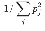 Weight distribution is measured by how many streams are used.
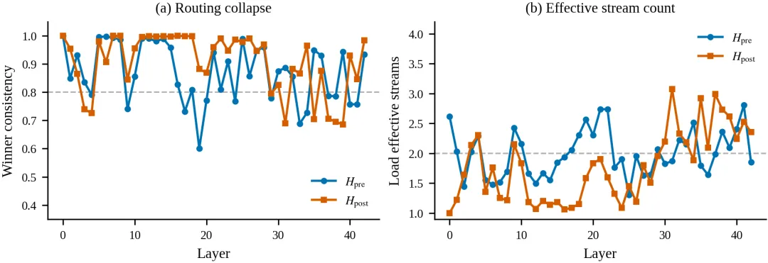
Figure 2: Left: dominant flow consistency; right: effective flow quantity. Each point combines the statistical results of the same Attention and FFN substrate.
In Figure 2, the read-map dominance stream consistency is 0.871, and the write-map consistency is 0.905. That is, within a given sublayer, most tokens often share the same dominance stream.
At the same time, the reading mapping corresponds to an average of 1,998 effective streams and the writing mapping to 1,775 streams. This indicates that although the architecture provides four streams, a typical Attention or FFN calculation actually places the main weight on only about two streams.
The above statistics describe routing patterns within a single sublayer. Figure 3 further shows the average read-write weight of streams in different sublayers.
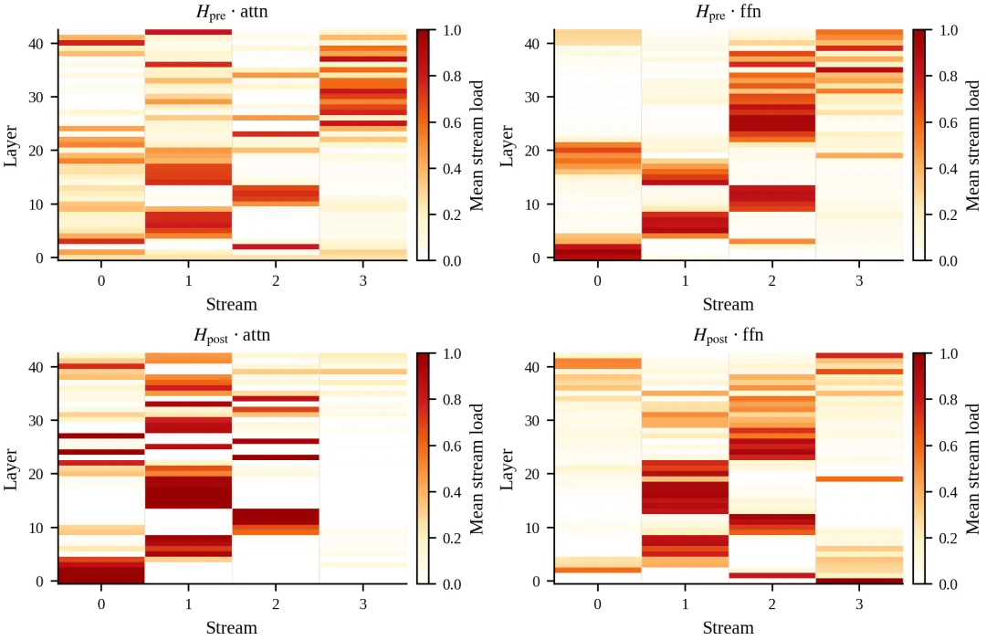
Figure 3 Average flow loads at four classes of locations. High load areas form continuous depth ranges, but the dominant flow changes with layers, sublayer types and read-write mapping.
Similarity between residual flows
A question that needs to be examined further is whether the representation of the four streams has tended to be similar, so that the model only needs to concentrate on a few of them. We calculated the residual similarity between the hidden states of the four streams in each Attention or FFN sublayer and compared the total of the six groups to two, see Figure 4.
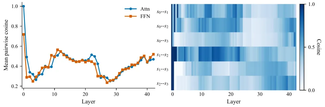
Figure 4 shows the resemblance of the four residual flows between the two as the depth changes. The left-hand graph shows the average value of the six groups of flows, and the right-hand graph shows the groups of flows respectively. The deeper the color, the higher the resemblance.
In Figure 4 to the left, the four residual streams at the model entrance have a residual similarity of 1, because they are replicated by the same input representation. After the first Transformer layer, the representation of the streams begins to differentiate; in the subsequent network, the average line similarity of the six group streams pairs is between 0.235 and 0.564, with an overall average of 0.404.
The graph on the right shows six groups of flow pairs separately, with each row corresponding to a group of flow pairs. The deeper the color, the higher the resynchronous similarity.
However, whether the direction of representation is the same and whether a specific read-write path is necessary are two different questions. Even if the direction of representation of a stream is different from other streams, when assigned a smaller read-write weight, the output of the model may still be limited.
Mixed residual mapping changes with depth
We used the average absolute deviation of the residual mixed matrix and the unit matrix to measure the cross-flow mixing intensity of each sublayer:

When a unit matrix, the four streams pass along the residual path respectively. Figure 5 gives the average value of each Attention and FFN substrate on the calibrated token.
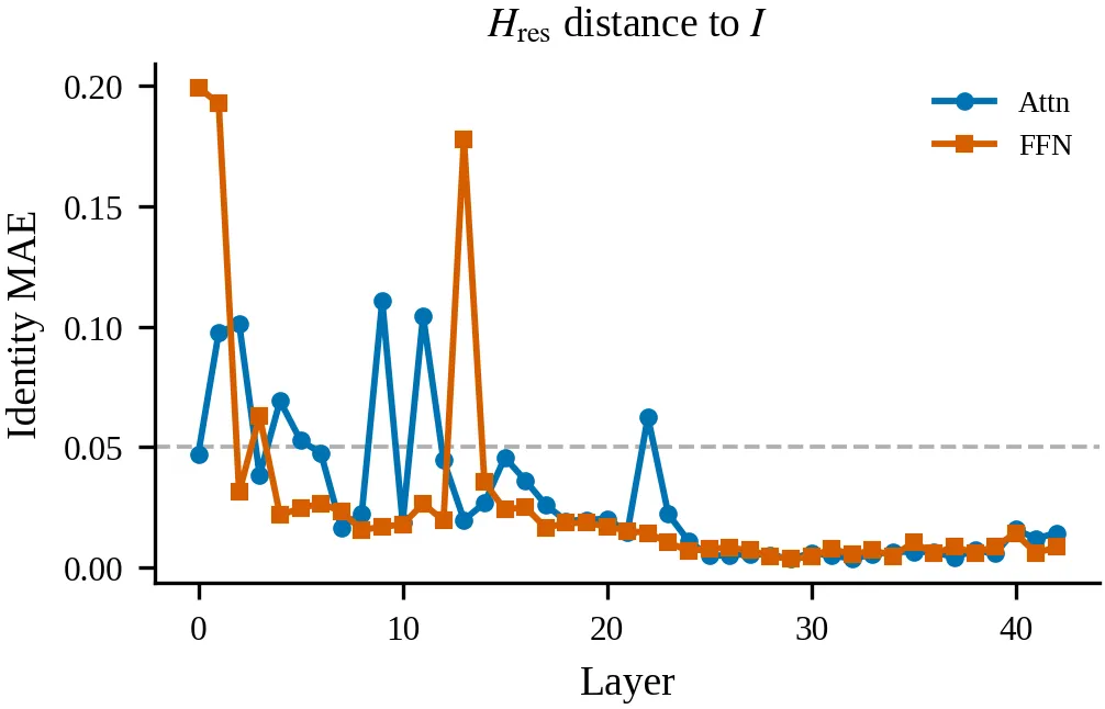
Figure 5 shows the deviation of the unit matrix of the Attention and FFN substrate, each point being the average value on the calibrated token.
Figure 5 shows that larger deviations occur mainly in the first half of the model. After the 22nd layer, the residual mixed matrix gradually approaches the unit matrix. In the 40 sub-layers of the 23rd layer, there are 32 sub-layers with deviations below 0.01.[4] Figure 6 gives the average residual mixed matrix of the 0th layer, 21st layer and 22nd layer, 42nd layer, respectively:
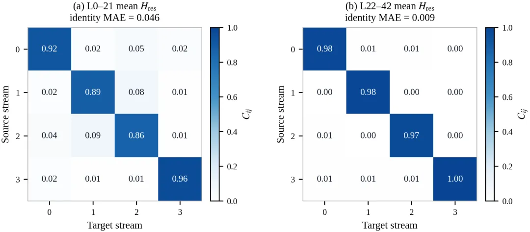
Figure 6 shows the average residual mixed matrix of layers 0-21, and 22-42.
This more intuitively illustrates this difference in depth: the mean matrix of layer 021 can still be seen in non-contrast weight; the mean matrix of layer 2242 is close to the unit matrix.
Read-write path cuts and replaces mixed mapping with residual mapping
Read, write, cut paths
For each token and each sublayer, we retain the maximum weight in reading and writing maps, respectively.
The path is then scaled down to the ratio of the remaining weights, so that the weight is the same as before the cut.
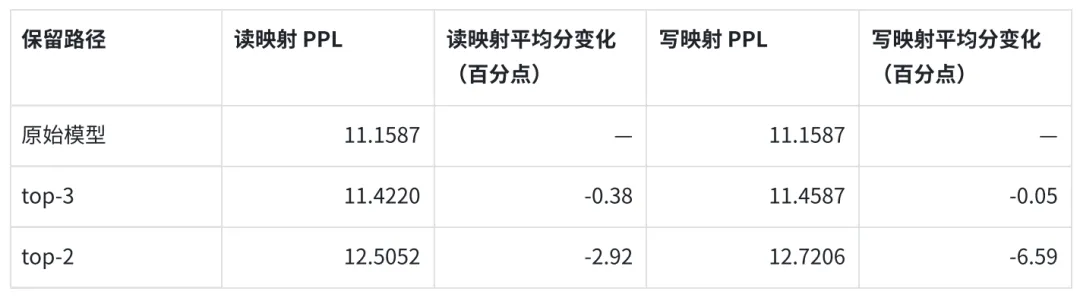
While maintaining the top-3, the read-write path cutting has less impact on PPL and the six task averages. Further cutting to the top-2 increases the change in the two indicators significantly, with the mapping cutting having greater impact. Thus, one path with the least weight can be approximately removed.
Remains of mixed mapping
We'll replace the residual mixed matrix in the depth range. We'll also use the average matrix on each shallow sublayer on the C4 calibrated cluster token to replace the matrix that the sublayer originally generated dynamically, and we'll look at the role of each token-by-token change separately.
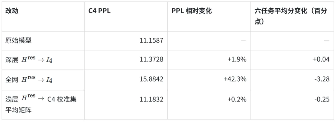
After replacing the deep residue mixed matrix, the PPL increased by 1.9%, the six-task average variation by +0.04 percentage points; after replacing the entire residual mixed matrix, the PPL increased by 42.3%, the six-task average decreased by 3.28 percentage points. This indicates that the direct cross-flow mixing effect of closing deep residue is less, but changing the entire network into a unit matrix will result in a significant performance decline.
After fixing the shallow layer to the average C4 matrix of each sublayer, the PPL increased by 0.2%, and the six-mission average decreased by 0.25 percentage points. This intervention fixed the shallow layer's cross-flow mix, illustrating the limited additional effect of the token-by-token change.
Figure 7 further lists the change in scores for each task:
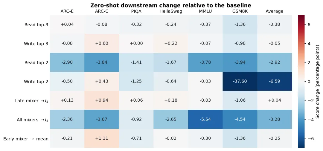
Figure 7 shows a change in the zero sample score of the interventions relative to the original model, in units of percentage points. To highlight the range of common changes, the color stages are intercepted at ±7 and the genome numbers retain the true change value.
Discussion: Simplification of the structure of multi-fluid residues
On a read-write route, some low-weight paths can be removed, but continuing to increase the cutting intensity will lead to a decrease in performance. Therefore, the density of the read-write route can be explored while maintaining the multi-stream structure and appropriately reduced. Whether such a design can match the performance of the model with computational efficiency needs to be retrained and evaluated in the corresponding architecture.
Residual mixed mapping exhibits significant differences in depth: after deep replacement to uniform mapping, the model performance changes less; the shallow layer still needs cross-flow mixing, but the effect of the token-by-token variation within the same sublayer is limited. Thus, the dynamics of the residual mixed mapping can be explored as the depth changes, without the need for the same mechanism in all layers. Two more recent multi-flow models have adopted a simpler residual path: Tencent Hy4-preview's identity Hyper-Connections (iHC) will be fixed as a matrix, while Qwen3.8-Flash-Next Gated Residual will directly remove this mapping.