The authors are from Lehigh University, the University of British Columbia and the Vector Institute. The first co-author is Lehigh University PhD students Dingjie Song and Zhiling Yan, and the communications author is Lichao Sun, an assistant professor at Lehigh University.
To let the big model "think a little more" today is almost equivalent to having it write a few more words: Mr. into a chain of thought and then give an answer.
But in many real-world systems, the model has only one choice: which tool the request is given to, which category the text belongs to, which one the candidate moves to select.
The decision-making model is fast, but the calculation quantity is dead in training. Simple questions and difficult questions take the same amount of time to calculate, and difficulty encounters can't be thought of for a moment. Another way is to have the model write the reasoning first and answer the answer, so that each question has to pay for the reasoning text, and simple questions are no exception.
Meanwhile, the Circular Transformer has recently become a hot spot again in the industry. The original Circular Language Model, represented by Ouro in Seed bytes, allows the same set of layers to be computed repeatedly during the pre-training phase, putting "thinking" into a hidden state.
Can a decision-making model do the same thing with "multi-circles"?
Recently, researchers from institutions such as Lehigh University have proposed Lev, a decision-making model for deepening thinking with a loop rather than a token. Lev reads the probability of an option after each round, and the rounds are trained together, so the same weight can be answered at any depth; a lightweight stopper then decides several rounds by title. The authors call this method System 1.5: retain System 1 to give the decision interface directly, and can spend more on the problem as System 2 does.
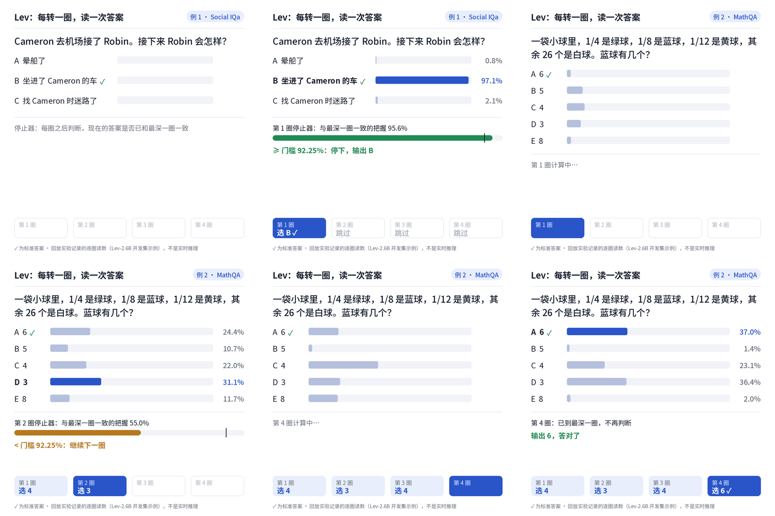
Lev responds round-by-round, redrawing the round-by-round readings according to the project's homepage records, relaying experimental data, not real-time reasoning: Example 1 Round 1 selects the correct answer B, and the stop-motion determination can be stopped; Example 2 Round 1 selects 4, and Round 4 selects the correct answer 6.
From a task format perspective, Lev can be seen as a standalone open source implementation of OpenAI Decisions-style text decision-making, with a "deep spin" added. The "model" here refers only to the task format: given inputs and candidates, the probability of each option's output. Lev is based on the open Ouro, Nanbeige baseline and Kev implementation, without repeating OpenAI's model weight, internal architecture or API, or performance measurements with any of its products.
In an open JevBench 231 question, the same Lev-2.6B checkpoint was raised from 63.2% of a circle to 76.2% of a four-circle, an increase of 13.0 percentage points.
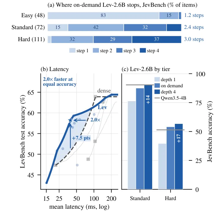
Chart 1: (a) The number of rounds used in JevBench for each difficulty grade below the required depth of Lev-2.6B; (b) LevBench locks the accuracy and latency on the test; (c) Lev-2.6B the accuracy of the rounds, on demand, of the four rounds on the standard and difficulty problems, controlling Qwen 3.5-4B trained for the same data.
Lev: Thinking Fast and Deep with Looped Decision Models
Link to the paper:https://arxiv.org/abs/2610.20951
The code is:https://github.com/OpenLAIR/lev
Models and data:https://huggingface.co/collections/songdj/lev
The main page of the project:https://openlair.github.io/lev/
Why do decision-making models need to be deepened on demand?
The authors first used two open decision models, Kev-0.8B and Kev-4B, to make a case-by-case comparison. Both of them were trained from the same data source, and in JevBench's 231 open questions, Kev-4B answered Kev-0.8B multiple-choice questions in 28 ways, all 28 of which came from standard questions and problems: the two models of simple questions would have been completely correct.
More importantly, the two models differed only in the results of 42 path queries, but Kev-4B spent more on the parameters and calculations on each of them. If Kev-0.8B reliably selected at least half of its uncertain questions for Kev-4B, the accuracy would almost equal the total number of Kev-4B responses.
In other words, extra computation is only useful on a few subjects, and a cheap initial reading can find these subjects.
The authors examine three types of calculations one by one:
Grade: assign uncertain questions to large models. But the average delay for Kev-0.8B is already 79 ms, andKev-4B is 108 ms, and the translated questions are to be read over and over again, spending more time than directly using the large model, and more time deploying a single model.
Generate reasoning text: On two open-source Jev services on the same 26B baseline, open thinking can increase the accuracy of the difficulty by 9 to 13 points, but the difficulty median takes three to four times the original time, and simple questions also pay for reasoning text.
On the bottom of the Kev-0.8B Qwen3.5-0.8B, the authors took the middle eight layers into a loop with gate controls and trained them according to the Kev formula. The resulting accuracy rate varied by less than half a point; improving the gate control learning rate, multiple turns, and widening the loop blocks were not helpful, the gate controls were always close to zero, and the loop was almost unopened.
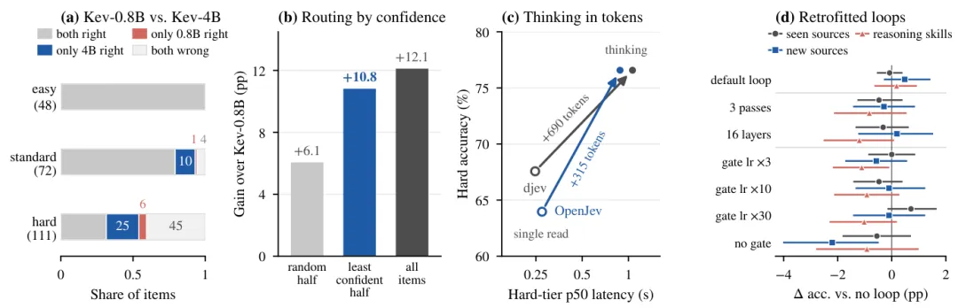
Chart 2: ((a) Kev-0.8B and Kev-4B results on each of the questions on JevBench; ((b) Kev-4B answers half randomly, improves relative to Kev-0.8B when not knowing at least half or all of the questions; ((c) reads and generates the same underlying reasoning on the same basis; ((d) changes in the accuracy after the Qwen3.5-0.8B add-on cycle.
The latter directly determines Lev's design: instead of teaching models to use cycles in decision-making training, it's better to learn to start at the bottom of the cycle from a pre-train.
How to Lev: Read the answer every turn
Lev interfaces with Kev's decision-making model. A request contains a state (such as a conversation or a document) and several questions, each of which lists its candidates. All content is packaged into a sequence with block causal disguise to allow each question to see only the state and itself, so that the state is encoded only once, and each question is answered as a separate question.
The difference lies at the bottom: Lev replaced the native loop language model Ouro or Nanbeige 4.2 with the same set of decoding layers. Run R repeatedly, and after each round, the same pointer head reads the hidden state of each option's endpoints and <decide> locations, producing an option probability.
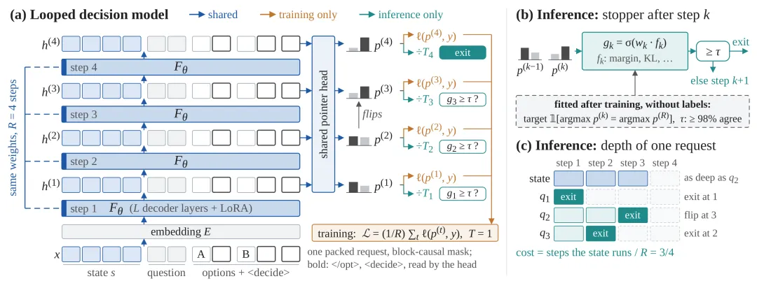
Figure 3: Lev's structure (e.g. 4 circles) (a) The same set of decoded layer cycles R times, with a shared pointer head that reads an option once per circle; (b) After each circle, the stop predicts whether the current answer is consistent with the deepest circle; (c) Each question exits at its own depth, and the state counts only the depth required for the deepest question.
When training, the pointer head and the LoRA adapter are shared between the laps, and the losses are averaged over all the laps, so each depth is trained as a decision model available rather than just the last lap.
This brings two direct benefits. First, the first t-circle relies only on the front circle, and with k-circles only the first k-circle is served, costing about the full depth of k/R. Second, "recalculate a circle" is to continue to calculate from the hidden state of the previous circle, requiring no re-reading, which is exactly what a hierarchy cannot do.
In addition, low-level and deep-level readings vary in calibration, with the authors adapting a temperature for each depth separately. Temperature scaling does not change the prediction options, so it does not affect accuracy.
When should we stop?
It predicts "consistent with the deepest circle".
It's not "yes".
After reading each circle, the next question is: How many circles are there in each question?
The common practice of early withdrawal is to select a confidence threshold on labeled data when confidence is high enough to stop. The authors found that this rule migrated poorly in decision models for two reasons:
Low-level reading is overconfidence in new data. Lev-2.6B stopped the topic for a while, with 94.8% correct on the calibration set, and only 78.9% correct on the new data source Kev-Transfer, whereas confidence is almost the same.
Confidence cannot be seen in the error "One more round can be corrected". The AUROC of confidence difference between errors is 0.67 to 0.83, but the difference between "multiple rounds can be corrected" and other topics is only 0.46 to 0.61, almost random.
Thus, Lev's stopwatch changed the prediction goal: in the k-circle, predict whether the current answer is already consistent with the answer to the deepest circle. It is a logical regression at each depth, characterized only by the reading of the current circle and the previous one: the highest probability, the gap between the first two, the regression of the chemistry, whether the answer has changed, the KL scattering distribution of the two circles, etc.
The advantage of this goal is that the standard answer is the model's own deepest answer, and the matching stop and the selection threshold do not require any artificial labeling. The threshold takes a minimum value that makes at least 98% of the final answer consistent with the deepest answer. When deployed, the stop can be directly calibrated using unlabelled requests from its own business.
Experiments: One Weight, Multiple Work Points
The authors constructed Lev-1.4B (Ouro-1.4B), Lev-2.6B (Ouro-2.6B, 4 rounds) and Lev-3B (Nanbeige 4.2-3B, 2 rounds) on the bases of the three cycles. Nanbeige pre-training loses only in the last round to test whether Lev relies on the controlled middle circle during pre-training.
The control group was Qwen3-1.7B, Qwen3.5-2B, and Qwen3.5-4B, three non-recycled (dense) models using the same 31,329 training data and formula as Lev (LoRA rank 16, training round).
In terms of evaluation, the authors first set the formula and stop design on three modules, and then read two held-out test sets: one covering five application areas, Kev-Breadth covering 14 data sets that had never been trained; the other is the author's self-built LevBench, which freezes before any model is read, and the difficulty file goes from a new topic from the training source to a completely unseen data set.
Finding 1: The same weight, the deeper the depth, the lower the yield.
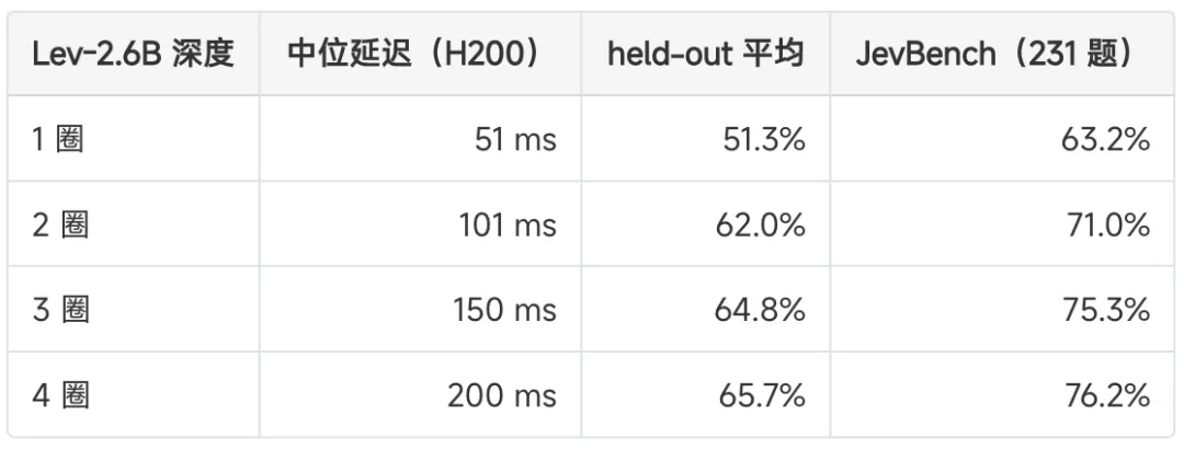
This trend was observed in all three test sets. A 13.0 percentage point improvement on the first lap to the fourth lap on JevBench (95% confidence interval from 7.4 to 19.0) was observed. Most of the gains came from the first additional lap: Lev-2.6B's hold-out increased from an average of 51.3% to 62.0%, with a maximum of 1 point on the fourth lap.
The further away from the training data, the deeper the effect: on the training data source, a circle to four circles increases about 7 points; on the other four test sets further away from the training data, it increases to 9.0 to 19.5 points.
Figure 2: Most computations are devoted mainly to complex problems.
On the JevBench, Lev-2.6B ranges from one circle to four circles, with a polynomial of 10 for 72 standard questions, and a polynomial of 19 for 111 problems; simple questions are almost perfect at every depth.
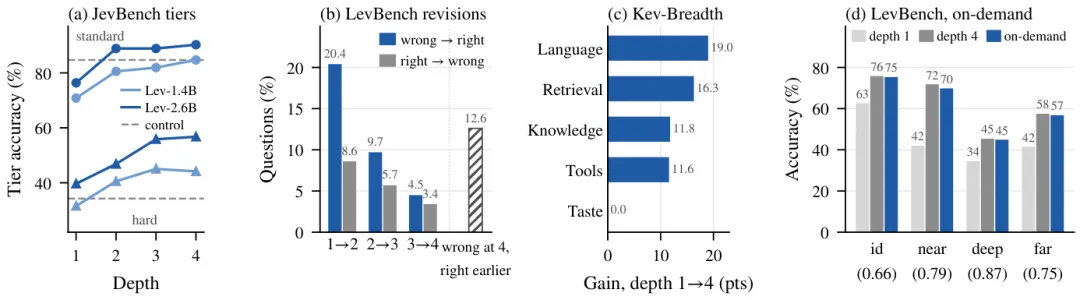
Paper Chart 5: Where depth works. (a) The accuracy of JevBench standard questions and problems; (b) The topics modified between adjacent circles on LevBench; (c) The improvement of Kev-Breadth from one circle to four circles in each application area; (d) The accuracy of each LevBench difficulty file and the cost of depth on demand.
In LevBench, the first additional round-up was 20.4% of the questions and 8.6% of the questions were incorrect. Another 12.6% of the questions were correct, with some shallower round-ups being correct, and the deepest round-ups being incorrect, so that stoppers "consistent with the deepest round" could not solve these questions. Different tasks also have different benefits: in Kev-Breadth, deep language comprehension tasks are improved by 19.0 points, while there is no benefit in humor and color preference tasks.
Findings 3: Less than 15% to 24% of the required depth, and less than 1 point of accuracy loss.
In two held-out test sets, the stoppers used only 76% to 85% of the calculation of the deepest circle, with an accuracy of less than 1 point (0.3 to 0.8 points) compared to the deepest circle.
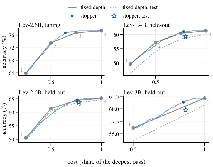
Figure 6: Accuracy rate and computational costs. Gray for each fixed depth and its connecting lines (Fixed Depth Front), blue for the deviation of the moving stop; null and asterisk for the result of the locking test.
The stop can't see the difficulty of the title completely, but automatically spends more rounds on the difficulty: on JevBench, the Lev-2.6B on demand averages 1.2 and 2.4 and 3.0 rounds respectively on the simple, standard and difficulty problems.
The authors also reported the limits of this gain. Compared to "the mixed use of fixed depths at equal cost", the advantages of the required depth are not great: Lev-2.6B is only 0.2 points higher on the held-out, Lev-3B is 1.0 points higher. The reason is that the front of the Ouro model itself is thick, and the first additional circle takes most of the gain.
It should be pointed out that the "minor computation" here is the computation of the circuitry of offline statistics. To convert it into online throughput or delayed gain, it is also necessary for the service end to support packaging and scheduling of different depth requests, which is not within the scope of this article.
Discover 4: The key is not the characteristics of the stop, but the calibration of the target traffic.
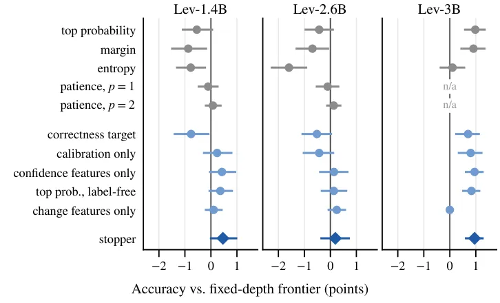
Figure 8: The accuracy of each stop rule is relatively poor at fixed depth fronts at the same cost. 95% confidence interval. Gray is the common early-return rule, and light blue is the meltdown of the stop device.
For the Ouro model, the confidence rule for adjusting thresholds for labeled data, as well as the rule for early withdrawal based on gaps, gaps and patience, cannot exceed the fixed depth forefront. As long as, like stoppers, a simple maximum probability threshold can be reached with a stopper of only 0.2 points if the thresholds are chosen as "consistent with the deepest answer" in a non-label target request.
Not much unlabeled data is needed: for every 500 queries, the Lev-2.6B equals less than 0.2 points to the total fit.
Findings 5: In low latency ranges of up to 50 ms, small Lev is more accurate than dense models and ranges with delay.
Figure 10: LevBench locks the accuracy rate and average latency on the test. Real lines connect to each fixed depth of the same Lev checkpoint, with star numbers at the desired depth; null lines are best dense models or scales, with numbers at the desired Lev and its gaps.
At a delay of 39 to 46 ms, the Lev-1.4B and Lev-3B on demand are 7.0 to 8.8 points higher than the only levels that can be reached at this delay, and 5.4 to 7.5 points higher than the best dense solutions.
The author also makes the conditions clear:
Part of the advantage comes from the dense scheme itself: there is no dense model between 22 and 79 ms.
Delays are measured on a single H200, bf16, one at a time, without convergence algorithms, graph capture or state caching, all systems are peer-to-peer.
According to the floating-point calculations, each Lev model is evenly matched or worse than the dense scheme, since each circle must run the entire base.
Lev-2.6B at about 150 ms is no better than using Kev-4B directly.
Similarly, Lev can match a larger model with fewer parameters: Lev-3B is evenly matched to Qwen 3.5-4B on JevBench, Lev-2.6B is evenly matched to open Kev-4B (76.2% to 75.8%, no significant difference).
Some observations on training
Compared to the Ouro-2.6B model with only a single deep-train, the Lev-2.6B was level on 2 laps and 4 laps, with a maximum of 1.3 points behind on 1 lap; training only the last lap would render the shallow layers completely unusable.
More data mainly reinforced the shallow layer. The training data expanded from 310,000 to 120,000, the level of accuracy of a lap held-out by Lev-2.6B increased from 50.5% to 62.9%, the deepest lap increased from 65.3% to 73.0%, and the cost of depth on demand decreased from 0.76 to 0.63.
LoRA is superior to full-parameter modulation. For the Ouro model, full-parameter modulation drops the deepest circle by 1.3 to 1.9 points and loses the relative edge advantage.
Limitations
The paper study's loop base is between 1.4B and 3B, a scale that is currently publicly available, and a larger loop model can push the depth curve how far and remains to be verified. JevBench's results are based on only 231 open questions. The cost of the required depth is calculated by the number of circuits, to be converted into a real-time logical system that can pack different depth requests for services. Delay measurements do not optimize any service end, and optimization services for the loop model and dense model remain for the future.
Summary
Lev turned the depth of the loop into a setup that was decided only in service: the same decision model weight could be swapped between latency and accuracy by subject, without having to deploy a model for each budget. Experiments showed that the improvement in depth was mainly due to the difficulty; using "consistent with the deepest answer" as a goal, stoppers calibrated on non-label requests could assign more computation to the difficulty without seeing the difficulty.
The authors argue that there are two directions to follow: whether the design can salvage the 12.6% problem-stop target of "shallow-level answering, deep-level answering errors" and thus exceed the accuracy of the deepest circle; and whether the gains of the problem-testing on the larger loop base will increase with scale.
The papers, the code, the three models and the three datasets have all been made public. The datasets are sub-sets that have been filtered according to the terms of redistribution from each source, and cannot be accommodated by the source attached reconstruction instructions.
Introduction by the author
Dingjie Song, first co-author: PhD student at Lehigh University.
Zhiling Yan (co-author number one): PhD student at Lehigh University
Yuxuan Zhang: PhD student at the University of British Columbia, Vector Institute.
Lichao Sun ((communication author): Assistant Professor at Lehigh University, topic group homepage

© THE